MySQL 8.0.2 introduces SQL window functions, or analytic functions as they are also sometimes called. They join CTEs (available since 8.0.1) as two of our most requested features, and are long awaited and powerful features. This is the first of a series of posts describing the details. Let’s get started!
Introduction
Similar to grouped aggregate functions, window functions perform some calculation on a set of rows, e.g. COUNT or SUM. But where a grouped aggregate collapses this set of rows into a single row, a window function will perform the aggregation for each row in the result set, letting each row retain its identity:
Given this simple table, notice the difference between the two SELECTs:
mysql> CREATE TABLE t(i INT);
mysql> INSERT INTO t VALUES (1),(2),(3),(4);
mysql> SELECT SUM(i) AS sum FROM t;
+------+
| sum |
+------+
| 10 |
+------+
mysql> SELECT i, SUM(i) OVER () AS sum FROM t;
+------+------+
| i | sum |
+------+------+
| 1 | 10 |
| 2 | 10 |
| 3 | 10 |
| 4 | 10 |
+------+------+
In the first select, we have a grouped aggregate; the there is no GROUP BY clause, we we have an implicit group containing all rows. The values of i get summed up for the group, and we get a value of 10 as a result row.
For the second select, as you can see, every row from t appears in the output, but each rowhas has the value of the sum of all the rows.
The crucial difference is the addition of the OVER () syntax after the SUM(i). The keyword OVER signals that this is a window function, as opposed to a grouped aggregate function. The empty parentheses after OVER is a window specification. In this simple example it is empty; this means default to aggregating the window function over all rows in the result set, so as for the grouped aggregate, we get the value 10 returned from the window function calls.
In this sense, a window function can be thought of as just another SQL function, except that its value is based on the value of other rows in addition to the values of the for which it is called, i.e. they function as a window into other rows.
Now, it is possible to do this calculation without window functions, but it is more complex and/or less efficient, i.e.
mysql> SELECT i, (SELECT SUM(i) FROM t) FROM t;
+------+------------------------+
| i | (SELECT SUM(i) FROM t) |
+------+------------------------+
| 1 | 10 |
| 2 | 10 |
| 3 | 10 |
| 4 | 10 |
+------+------------------------+
that is, we use an explicit subquery here to calculate the SUM for each row in “t”. It turns out that the functionality in window functions can be expressed with other SQL constructs, but usually at the expense of both clarity and/or performance. We will show other examples later where the difference in clarity becomes starker.
Window functions come in two flavors: SQL aggregate functions used as window functions and specialized window functions. This is the set of aggregate functions in MySQL that support windowing:
COUNT, SUM, AVG, MIN, MAX, BIT_OR, BIT_AND, BIT_XOR,
STDDEV_POP (and its synonyms STD, STDDEV), STDDEV_SAMP,
VAR_POP (and its synonym VARIANCE) and VAR_SAMP.
The set of specialized window functions are:
RANK, DENSE_RANK, PERCENT_RANK, CUME_DIST, NTILE,
ROW_NUMBER, FIRST_VALUE, LAST_VALUE, NTH_VALUE, LEAD
and LAG
We will discuss all of these in due course; but after reading this blog, you should be able to start experimenting with all of these right away by consulting the SQL reference manual.
But before we do that, we need to discuss the window specification a little. The following concepts are central: the partition, row ordering, determinacy, the window frame, row peers, physical and logical window frame bounds.
The partition
Again, let us contrast with grouped aggregates. Below, the employees record their sales of the previous month on the first day of the next:
CREATE TABLE sales(employee VARCHAR(50), `date` DATE, sale INT);
INSERT INTO sales VALUES ('odin', '2017-03-01', 200),
('odin', '2017-04-01', 300),
('odin', '2017-05-01', 400),
('thor', '2017-03-01', 400),
('thor', '2017-04-01', 300),
('thor', '2017-05-01', 500);
mysql> SELECT employee, SUM(sale) FROM sales GROUP BY employee;
+----------+-----------+
| employee | SUM(sale) |
+----------+-----------+
| odin | 900 |
| thor | 1200 |
+----------+-----------+
mysql> SELECT employee, date, sale, SUM(sale) OVER (PARTITION BY employee) AS sum FROM sales;
+----------+------------+------+------+
| employee | date | sale | sum |
+----------+------------+------+------+
| odin | 2017-03-01 | 200 | 900 |
| odin | 2017-04-01 | 300 | 900 |
| odin | 2017-05-01 | 400 | 900 |
| thor | 2017-03-01 | 400 | 1200 |
| thor | 2017-04-01 | 300 | 1200 |
| thor | 2017-05-01 | 500 | 1200 |
+----------+------------+------+------+
In the first SELECT, we group the rows on employee and sum the sales figures of that employee. Since we have two employees in this Norse outfit, we get two result rows.
Similarly, we can let a window function only see the rows of a subset of the total set of rows; this is called a partition, which is similar to a grouping: as you can see the sums for Odin and Thor are different. This illustrates an important property of window functions: they can never see rows outside the partition of the row for which they are invoked.
We can partition in more ways, of course:
mysql> SELECT employee, MONTHNAME(date), sale, SUM(sale) OVER (PARTITION BY MONTH(date)) AS sum FROM sales;
+----------+-----------------+------+------+
| employee | MONTHNAME(date) | sale | sum |
+----------+-----------------+------+------+
| odin | March | 200 | 600 |
| thor | March | 400 | 600 |
| odin | April | 300 | 600 |
| thor | April | 300 | 600 |
| odin | May | 400 | 900 |
| thor | May | 500 | 900 |
+----------+-----------------+------+------+
Here we see the sales of the different months, and how the contributions from our intrepid salesmen contribute. Now, what if we want to show the cumulative sales? It’s time to introduce ORDER BY.
ORDER BY, peers, window frames, logical and physical bounds
The window specification will often contain an ordering clause for the rows in a partition:
mysql> SELECT employee, sale, date, SUM(sale) OVER (PARTITION by employee ORDER BY date) AS cum_sales FROM sales;
+----------+------+------------+-----------+
| employee | sale | date | cum_sales |
+----------+------+------------+-----------+
| odin | 200 | 2017-03-01 | 200 |
| odin | 300 | 2017-04-01 | 500 |
| odin | 400 | 2017-05-01 | 900 |
| thor | 400 | 2017-03-01 | 400 |
| thor | 300 | 2017-04-01 | 700 |
| thor | 500 | 2017-05-01 | 1200 |
+----------+------+------------+-----------+
We are summing up sales ordered by date: And as we can see in the ‘cum_sales’ column: row two contains the sum of sale of row one and two, and for each employee the final sale is, as before, 900 for Odin and 1200 for Thor (a big hammer is a presumably a persuasive sales argument).
So what happened here? Why did our adding an ordering of the partition’s row lead to partial sums instead of the total for each row, as we had before?
The answer is that the SQL standard prescribes a different default window in the case of ORDER BY. The above window specification is equivalent to the explicit:
that is, for each sorted row, the SUM should see all rows before it (UNBOUNDED), and up to and including the current row. This represents an expanding window frame, anchored in the first row of the ordering.
So far, so good. However, there is a subtle point lurking here: Watch what happens here:
mysql> SELECT employee, sale, date, SUM(sale) OVER (ORDER BY date) AS cum_sales FROM sales;
+----------+------+------------+-----------+
| employee | sale | date | cum_sales |
+----------+------+------------+-----------+
| odin | 200 | 2017-03-01 | 600 |
| thor | 400 | 2017-03-01 | 600 |
| odin | 300 | 2017-04-01 | 1200 |
| thor | 300 | 2017-04-01 | 1200 |
| odin | 400 | 2017-05-01 | 2100 |
| thor | 500 | 2017-05-01 | 2100 |
+----------+------+------------+-----------+
We removed the partitioning, so we can get accumulated sale over all our salesmen, and true enough, the total is 2100 on the last row as expected. But, so has the second but the last row! Similarly, row one and two have the same value, as do three and four. But, hold on, you’d be forgiven for asking: I thought you just said we’d get a window to and including the current row?
The clue lies in the keyword RANGE above: windows can be specified by physical (ROWS) and logical (RANGE) boundaries. Since we order on date here, we see that the rows having the same date have the same sum. That is, actually our window specification logically reads
(PARTITION by employee ORDER BY date
RANGE BETWEEN UNBOUNDED PRECEDING AND CURRENT ROW /* and its peers */)
that is, the window frame here consists of all rows earlier in the ordering up to and including the current row and its peers; that is, any other rows that sort the same given the ORDER BY expression. Two rows with equal dates obviously sort the same, hence they are peers.
If we wanted the cumulative sum to increase per row, we’d need to specify a physical bound:
mysql> SELECT employee, sale, date,
SUM(sale) OVER (ORDER BY date ROWS
BETWEEN UNBOUNDED PRECEDING AND CURRENT ROW) AS cum_sales
FROM sales;
+----------+------+------------+-----------+
| employee | sale | date | cum_sales |
+----------+------+------------+-----------+
| odin | 200 | 2017-03-01 | 200 |
| thor | 400 | 2017-03-01 | 600 |
| odin | 300 | 2017-04-01 | 900 |
| thor | 300 | 2017-04-01 | 1200 |
| odin | 400 | 2017-05-01 | 1600 |
| thor | 500 | 2017-05-01 | 2100 |
+----------+------+------------+-----------+
Note: the upper bound of the window frame (CURRENT ROW) is also default and can be omitted, as we do here:
mysql> SELECT employee, sale, date,
SUM(sale) OVER (ORDER BY date ROWS UNBOUNDED PRECEDING) AS cum_sales
FROM sales;
+----------+------+------------+-----------+
| employee | sale | date | cum_sales |
+----------+------+------------+-----------+
| odin | 200 | 2017-03-01 | 200 |
| thor | 400 | 2017-03-01 | 600 |
| odin | 300 | 2017-04-01 | 900 |
| thor | 300 | 2017-04-01 | 1200 |
| odin | 400 | 2017-05-01 | 1600 |
| thor | 500 | 2017-05-01 | 2100 |
+----------+------+------------+-----------+
The keyword ROWS signals physical boundaries (rows), whereas RANGE indicates logical bounds, which can create peer rows. Which one you need depends on your application.
Digression: if you omit an ORDER BY, there is no way to determine which row comes before another row, so all of the rows in the partition can be considered peers, and hence a degenerate result of:
(PARTITION by employee /* ORDER BY <nothing> */
RANGE BETWEEN UNBOUNDED PRECEDING AND CURRENT ROW /* and its peers */)
End of digression.
Determinacy
Let’s look again at the previous query:
mysql> SELECT employee, sale, date, SUM(sale) OVER (ORDER BY date ROWS UNBOUNDED PRECEDING) AS cum_sales FROM sales;
+----------+------+------------+-----------+
| employee | sale | date | cum_sales |
+----------+------+------------+-----------+
| odin | 200 | 2017-03-01 | 200 |
| thor | 400 | 2017-03-01 | 600 |
| odin | 300 | 2017-04-01 | 900 |
| thor | 300 | 2017-04-01 | 1200 |
| odin | 400 | 2017-05-01 | 1600 |
| thor | 500 | 2017-05-01 | 2100 |
| odin | 200 | 2017-06-01 | 2300 |
| thor | 400 | 2017-06-01 | 2700 |
| odin | 600 | 2017-07-01 | 3300 |
| thor | 600 | 2017-07-01 | 3900 |
| odin | 100 | 2017-08-01 | 4000 |
| thor | 150 | 2017-08-01 | 4150 |
+----------+------+------------+-----------+
We order the rows by date, but all rows share the same date as another row, so what is the order between those? In the above, it is not determined. An equally valid result would be:
+----------+------+------------+-----------+
| employee | sale | date | cum_sales |
+----------+------+------------+-----------+
| thor | 400 | 2017-03-01 | 400 |
| odin | 200 | 2017-03-01 | 600 |
| thor | 300 | 2017-04-01 | 900 |
| odin | 300 | 2017-04-01 | 1200 |
| thor | 500 | 2017-05-01 | 1700 |
| odin | 400 | 2017-05-01 | 2100 |
| thor | 400 | 2017-06-01 | 2500 |
| odin | 200 | 2017-06-01 | 2700 |
| thor | 600 | 2017-07-01 | 3300 |
| odin | 600 | 2017-07-01 | 3900 |
| thor | 150 | 2017-08-01 | 4050 |
| odin | 100 | 2017-08-01 | 4150 |
+----------+------+------------+-----------+
This time, Thor’s rows precede Odin’s rows, which is OK since we didn’t say anything about this in the window specification. Since we had a window frame with physical bound (“ROWS”), both results are valid.
It is usually a good idea to make sure windowing queries are deterministic. In this case, we can ensure this by adding employee to the ORDER BY clause:
(ORDER BY date, employee ROWS UNBOUNDED PRECEDING)
Movable window frames
One doesn’t always want to aggregate over all values in a partition, for example when using moving averages (or moving mean). To quote from Wikipedia:
“Given a series of numbers and a fixed subset size, the first element of the moving average is obtained by taking the average of the initial fixed subset of the number series. Then the subset is modified by “shifting forward”; that is, excluding the first number of the series and including the next value in the subset. A moving average is commonly used with time series data to smooth out short-term fluctuations and highlight longer-term trends or cycles.”
This is easily accomplished using window functions. For example, let’s see some more of the sales data for Odin and Thor:
TRUNCATE sales;
INSERT INTO sales VALUES ('odin', '2017-03-01', 200),
('odin', '2017-04-01', 300),
('odin', '2017-05-01', 400),
('odin', '2017-06-01', 200),
('odin', '2017-07-01', 600),
('odin', '2017-08-01', 100),
('thor', '2017-03-01', 400),
('thor', '2017-04-01', 300),
('thor', '2017-05-01', 500),
('thor', '2017-06-01', 400),
('thor', '2017-07-01', 600),
('thor', '2017-08-01', 150);
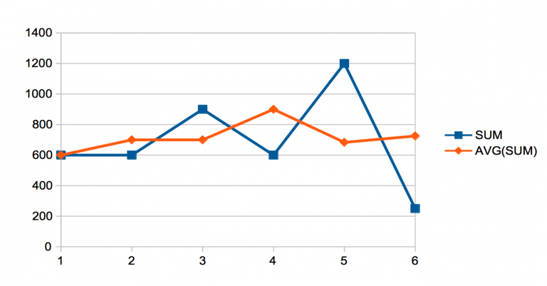
By averaging the current month with the previous and the next we get a
mysql> SELECT MONTH(date), SUM(sale),
AVG(SUM(sale)) OVER (ORDER BY MONTH(date)
RANGE BETWEEN 1 PRECEDING AND 1 FOLLOWING) AS sliding_avg
FROM sales GROUP BY MONTH(date);
+-------------+-----------+-------------+
| month(date) | SUM(sale) | sliding_avg |
+-------------+-----------+-------------+
| 3 | 600 | 600.0000 |
| 4 | 600 | 700.0000 |
| 5 | 900 | 700.0000 |
| 6 | 600 | 900.0000 |
| 7 | 1200 | 683.3333 |
| 8 | 250 | 725.0000 |
+-------------+-----------+-------------+
Or as shown in this graphic:

This can be expressed without window functions too:
WITH sums AS (
SELECT SUM(t2.sale) AS sum, t2.date FROM sales AS t2 GROUP BY t2.date )
SELECT t1.date,
( SELECT SUM(sums.sum) / COUNT(sums.sum) FROM sums WHERE MONTH(sums.date) - MONTH(t1.date) BETWEEN -1 AND 1)
FROM sales AS t1, sums
GROUP BY date
ORDER BY t1.date;
and even without CTEs
SELECT t1.date, SUM(sale),
( SELECT SUM(sums.sum) / COUNT(sums.sum) FROM
(SELECT SUM(t2.sale) AS sum, t2.date FROM sales AS t2
GROUP BY t2.date) sums
WHERE MONTH(sums.date) - MONTH(t1.date)
BETWEEN -1 AND 1
) AS sliding_avg
FROM sales AS t1
GROUP BY date
ORDER BY t1.date;
but it is rather more complex.
Conclusion
That’s all for now. Hopefully this gives you an idea of what window functions can be used for. In the next installment we’ll delve more into all the ways you can specify window frames, and introduce some of the specialized window functions. See you then!
And as always, thanks for using MySQL!